|
|
|
|
|
|
Abstract: We discuss two families of parameterized knots (polynomial and trigonometric) and include an interactive gallery of selected knots and their equations. We survey results related to parameterizations and suggest avenues for further investigation. Finally, we include an applet that graphs three-dimensional parametric curves to aid the interested reader in exploring additional parameterizations.
Knot Theory is a modern and active area of research, particularly appealing for its mathematical accessibility and visual aspect. However, knot theory also has applications of fundamental scientific significance: understanding DNA, for example. According to Sumners [18], "One of the important issues in molecular biology is the three-dimensional structure (shape) of proteins and deoxyribonucleic acid (DNA) in solution in the cell and the relationship between structure and function." The shape of DNA can be modeled by a curve. When DNA is knotted, difficulties in replication may result. Enzymes break apart and recombine DNA, affecting its structure; because the structure of DNA affects its function, understanding the types of knots formed by enzyme interactions is vital. An introduction to additional applications of knot theory can be found in [4].
Informally, we think of a knot as a curve in three-dimensional space. Formally, a knot is defined as the image of a continuous function \( f : [0, 1] \rightarrow \mathbb{R}^3 \) with the following properties:
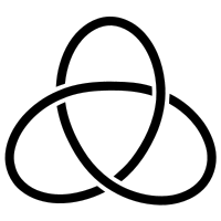
Typically, rather than stating the function \( f \), a knot is represented by a two-dimensional image called a knot diagram. A two-dimensional projection of a knot will typically appear to have double-points -- points where the curve intersects itself. However, a knot does not intersect itself; one strand of the curve is passing over the other strand of the curve. It is particularly important to know which strand passes over the other, and knot diagrams usually convey this information in one of two ways:
These two knot diagram styles are displayed in Figure 1 and Figure 2, two knot diagrams of a trefoil knot.
|
|
|
|
|
|
|
|
Two knots are defined to be equivalent and are said to have the same knot-type if one can be continuously deformed into the other while also continuously deforming the "ambient space" -- the space surrounding the knot. (This type of transformation is known as an ambient isotopy.)
Each knot-type may be embedded in three-dimensional space in many ways, and for each embedding there are many two-dimensional projections that may be converted to a knot diagram. Thus, it is not always clear when two knots have the same knot-type. As an example, Figure 3 contains a knot diagram very different than that of Figure 1, yet these two diagrams represent equivalent knots: the trefoil knot-type.
|
|
|
One of the fundamental problems in knot theory is to identify the knot-type of a knot from a given image. A standard method to show that two different diagrams represent the same knot-type is by the use of the three Reidemeister moves: ways in which a knot diagram may be altered locally while preserving the knot-type of the knot [21]. If two knot diagrams represent the same knot-type, then there is a sequence of Reidemeister moves that can be used to transform one knot diagram into the other.
Finding a sequence of Reidemeister moves to show that two knots are equivalent can be complicated. Furthermore, to demonstrate that two knots represent different knot-types using this method would require a proof that no such sequence of moves exist, an even more daunting task. This difficulty motivates the idea of invariants: mathematical objects (such as numbers or polynomials) associated to a given knot-type. If one calculates a particular invariant for two knots and obtains two different answers, then the knots have different knot-types. However, the converse is false: it is possible that different knot-types may have the same value for a particular invariant.
An example of a knot invariant is the crossing number: the smallest number of crossings that appear in any diagram of the knot. For example, the crossing number of the trefoil knot is 3; any diagram of the trefoil knot has at least 3 crossings. If a knot has a diagram with fewer than three crossings, then that knot is not a trefoil. Other examples of knot invariants include: tricolorability, unknotting number, stick number, bridge number, and the Jones polynomial [1]. Some of these invariants (such as tricolorability and the Jones polynomial) can be calculated from a single knot diagram.
Topics such as knot invariants and knot equivalence can be investigated directly from knot diagrams; for many purposes, it is not necessary to know a function whose image yields the knot under investigation. However, in this article we are particularly interested in parametric functions \( f(t) = \langle \, x(t), \, y(t), \, z(t) \, \rangle \) that yield knots, specifically parameterizations whose \( x, \, y, \) and \( z \) coordinates are given by relatively simple expressions in elementary functions: polynomial or trigonometric.
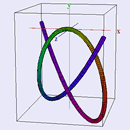
Parameterizations of knots yield another source of knot invariants, arising from a "simplest" parameterization of a knot-type, just as the crossing number invariant arises from a "simplest" knot diagram of a knot-type: one with a minimal number of crossings. For example, we will consider Shastri's trefoil polynomial knot (polynomial knots wil be defined in a later section). Shastri's trefoil is the image of the function \( f(t) = \langle \, x(t), \, y(t), \, z(t) \, \rangle \) where
\[ \begin{eqnarray} x(t) &=& t^3 - 3t \\ y(t) &=& t^4 - 4t^2 \\ z(t) &=& t^5 - 10t \\ \end{eqnarray} \]The coordinate functions are polynomials of degrees 3, 4, and 5; we say that this parameterization has "degree sequence" (3, 4, 5). Although there are many other parameterizations of trefoil polynomial knots, this is the smallest degree sequence possible; any polynomial knot with a smaller degree sequence is not a trefoil.
Minimal degree sequences are invariants of polynomial knots, and furthermore, the values of this invariant are related to values of other numerical knot invariants. Therefore, it is of interest to find particularly simple parameterizations for various knot-types, and to prove that a particular parameterization is the "simplest" with which the knot-type can be attained. Results of this nature will be mentioned in the sections that follow.
Parameterizations of knots also yield another notion of equivalent knots. For a given parameterization, we replace the numerical coefficients by variables; for example, we may replace the equations of Shastri's trefoil with the equations
\[ \begin{eqnarray} x(t) &=& t^3 + at \\ y(t) &=& t^4 + bt^2 \\ z(t) &=& t^5 + ct. \\ \end{eqnarray} \]Each choice of values for the coefficients \( a, b, \) and \( c \) yields a curve \( f(t) = \langle \, x(t), \, y(t), \, z(t) \, \rangle \). We consider the coefficient space: the set \( S \) of values \( (a, b, c) \in \mathbb{R}^3 \) such that the curve \( f(t) \) is a polynomial knot. Following Durfee and O'Shea [6], we call two parameterized knots path-equivalent if they are in the same connected component of \( S \). In other words, two parameterized knots are path-equivalent if we can start with the parameterization of one knot, continuously vary the coefficients until we obtain the parameterization of the other knot, and all the curves corresponding to intermediate values of the coefficients are also knots (that is, we never obtain a curve that intersects itself or has a zero tangent vector at some point).
It can be shown that parameterized knots which are path-equivalent are also equivalent in the standard sense: they have the same knot-type. A question of interest is to understand the coefficient spaces for various parameterizations; for instance, determine how many connected components exist in a given coefficient space, and to what knot-types each of the components correspond.
In what follows, we introduce two families of parameterized knots (polynomial and trigonometric) and include an interactive gallery of selected knots and their equations. We survey results related to parameterizations and suggest avenues for further investigation. Finally, we include an applet that graphs three-dimensional parametric curves to aid the interested reader in exploring additional parameterizations.
Since visualizing knots is vital to understanding and classifying them, producing galleries of knots with interactive three-dimensional graphics is a valuable endeavor.
Perhaps the most well-known software for this purpose is KnotPlot [16]. The KnotPlot website contains an excellent gallery of interactive three-dimensional graphics. An evaluation version of the KnotPlot program (with some features disabled) may be downloaded free of charge; the full version is available for purchase. The novel feature of the gallery in this article is the inclusion of parametric equations that generate the knot being viewed, and a parametric curve grapher that enables the reader to explore additional parameterizations.
The interactive three-dimensional graphics in this article are displayed using LiveGraphics3D, a Java applet written by Martin Kraus [5]. The applets should run on any Java 1.1-enabled internet browser. You may need to install the Java plug-in for your browser. Bugs in specific versions of certain browsers can occasionally prevent the LiveGraphics3D applet from initializing correctly. Often, reloading the page in your browser may fix this issue.
The basic applet controls are as follows:
A LiveGraphics3D applet is provided in Figure 4 for the convenience of the reader who wishes to familiarize themselves with the basic applet controls. For a complete list of applet controls, see the User Interface section of the LiveGraphics3D Documentation [10].
A polynomial knot is the image of a function \( f : \mathbb{R} \rightarrow \mathbb{R}^3 \) with the following properties:
Polynomial knots are not knots in the standard sense (as defined in the introduction), as they are not closed. For this reason, polynomial knots are sometimes referred to as "open-ended knots", "long knots", or "non-compact knots" in the literature. A technique called "one-point compactification" may be applied to convert polynomial knots into standard knots. This process can be easily visualized in the case of plane curves using stereographic projection, as we illustrate below; the case of space curves is completely analogous (but more difficult to visualize).
Let \( \mathcal{P} \) denote the \( xy \)-plane in \( \mathbb{R}^3 \), that is, the plane \( z = 0 \). Let \( \mathcal{S} \) denote a sphere of radius 1 centered at (0,0,2). (We choose this point for the center of the sphere for ease of visualization; in practice, the sphere is usually centered at (0,0,0) for algebraic simplicity.) Let \( N \) denote the north pole of the sphere. We define a function \( F : \mathcal{P} \rightarrow \mathcal{S} - \{ N \} \) as follows: for any point \( A \) in the plane \( \mathcal{P} \), the line containing \( A \) and \( N \) intersects the sphere \( \mathcal{S} \) at a point \( B \neq N \); let \( F(A) = B \). The function \( F \) is a bijection, and is formally known as "inverse stereographic projection". This function is illustrated in the applets contained in Figures 5, 6, and 7.
In Figure 5, a line is drawn from the red point in the plane to the north pole of the sphere; the projection of this point onto the sphere is displayed in blue. The red point may be moved around the plane by clicking and dragging with the left mouse button; the projection of this point onto the sphere will be automatically adjusted.
In Figure 6, a number of red points are drawn in the plane, arranged in a square, with one point in the center of the square. The projections of these points onto the sphere are drawn in blue. The red point in the center of the square may be moved around the plane by clicking and dragging with the left mouse button; the surrounding points and their projections onto the sphere will be automatically adjusted.
In Figure 7, a set of red points satisfying the \( x \) and \( y \) equations of Shastri's trefoil polynomial knot are drawn in the plane, and the projections of these points onto the sphere are drawn in blue. If the mouse pointer is positioned over the applet, an animation will be displayed: the image will rotate in three dimensions, and the line connecting points in the plane to their projections onto the sphere will trace through the points on the planar graph. The rotation of the image can be stopped by clicking once within the applet area. The animation of the line can be stopped and restarted by double-clicking within the applet area. Figure 7 illustrates the following fact: as the distance between a point \( A \) on the plane and the origin of the plane increases, the distance between the projection of \( A \) onto the sphere and the north pole of the sphere decreases. As the curve extends infinitely far away from the origin in the plane, the corresponding parts of the projection of the curve approach the north pole of the sphere. The union of the projection of the curve onto the sphere together with the north pole of the sphere is a closed curve; this result is called the "one-point compactification" of the curve.
Polynomial knots were introduced by Shastri in [15]. The knot-type of a polynomial knot is defined to be the knot-type of the one-point compactification of the polynomial knot (which is a knot in the standard sense). Using Weierstrass' approximation theorem, Shastri proved that for every knot type, there is a polynomial knot equivalent to it (after the one-point compactification process). As mentioned in the introduction, the minimal degree sequence for a polynomial knot is an invariant of interest. These values also yield bounds of other knot invariants, such as crossing number, bridge number, and superbridge number [6]. There is a concrete algorithm for finding polynomial knots equivalent to any given knot-type, although the degrees of the polynomials produced by this algorithm might not be minimal [12]. However, for polynomial knots that are equivalent to torus knots (defined in the next section), minimal degree sequences have been determined [13].
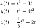
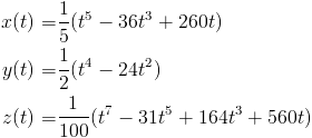
In the figures that follow, we include interactive three-dimensional graphics for five different polynomial knots. The polynomial knot equations were obtained from articles by Shastri [15] and Brown [5], with some coefficients scaled and/or slightly altered to produce visually appealing graphs. Polynomial knots are identified by their common name (when it exists) as well as by Alexander-Briggs notation \( C_N \), where \( C \) denotes the minimal crossing number in any projection of the knot, and \( N \) is an index number. A description of the basic applet controls are given in the above section, titled "Knot Software and LiveGraphics3D". To open the gallery page for a knot, click on either the knot's image or the knot's name in the table below.
|
|
|
|
|
A trigonometric knot is a knot as defined in the introduction, with the additional condition that in the function \( f(t) = \langle \, x(t), \, y(t), \, z(t) \, \rangle \), the coordinate functions \( x, y, \) and \( z \) are written in terms of trigonometric functions.
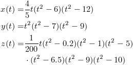
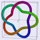
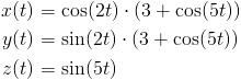
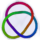
Possibly the most well-known type of trigonometric knots are torus knots, knots that lie on the surface of a torus. Torus knots are uniquely identified by a pair of relatively prime integers, \( p \) and \( q \), which specify the number of times the curve wraps around the torus in the longitudinal direction and the meridianal direction, respectively; such a knot is called a \( (p, \, q) \)-torus knot. Parametric equations for such a knot are given by: \[ \begin{eqnarray*} x(t) &=& \cos(qt) \cdot (3 + \cos(pt)) \\ y(t) &=& \sin(qt) \cdot (3 + \cos(pt)) \\ z(t) &=& \sin(pt) \end{eqnarray*} \] A \( (p,q) \)-torus knot is equivalent to a \( (q,p) \)-torus knot, and so we assume (without loss of generality) that \( p > q \). Realizing that a knot is a \( (p,q) \)-torus knot yields invariant information for that knot. For example, a \( (p,q) \)-torus knot has bridge number \( q \) (see [17]) and crossing number \( p(q - 1) \) (see [14]).
Another class of trigonometric knots are Lissajous knots, introduced in 1994 [2]. A knot is called Lissajous if it has a parameterization of the form \[ \begin{eqnarray*} x(t) &=& \cos(n_x \cdot t + \phi_x) \\ y(t) &=& \cos(n_y \cdot t + \phi_y) \\ z(t) &=& \cos(n_z \cdot t + \phi_z) \\ \end{eqnarray*} \] where the frequencies \( n_x, n_y, \) and \( n_z \) are positive integers and the phase shifts \( \phi_x, \phi_y, \) and \( \phi_z \) are real numbers. In [2], a particular invariant (the Arf invariant) of such knots is calculated and used to show that knots such as the trefoil knot, the figure-eight knot, and the cinquefoil knot have no such parameterization. In the same article, Lissajous parameterizations are given for many knots with crossing number between 5 and 10.
Naturally, one wonders if equations of other knots can be obtained if each coordinate function is a linear combination of cosine functions (rather than just a single cosine function). Such knots have a parameterization of the form \[ \begin{eqnarray*} x(t) &=& A_{x,1} \cos(n_{x,1} t + \phi_{x,1}) + \cdots + A_{x,i} \cos(n_{x,i}t + \phi_{x,i}) \\ y(t) &=& A_{y,1} \cos(n_{y,1} t + \phi_{y,1}) + \cdots + A_{y,i} \cos(n_{y,i}t + \phi_{y,i}) \\ z(t) &=& A_{z,1} \cos(n_{z,1} t + \phi_{z,1}) + \cdots + A_{z,i} \cos(n_{z,i}t + \phi_{z,i}) \\ \end{eqnarray*} \] and are referred to as both Harmonic knots and Fourier-\( (i,j,k) \) knots in the mathematical literature. By results on approximating functions with Fourier series, it can be shown that for every knot-type, there is a Fourier-\( (i,j,k) \) parameterization that yields a knot of that knot-type. The minimal values of \( i, j, \) and \( k \) that yield a parameterization of a given knot-type are an invariant of that knot-type, and are related to other knot invariants, such as the crossing number and superbridge number [19], [20]. Trigonometric identities are used to convert the standard equations of a torus knot into a Fourier-(3,3,1) parameterization in [8], where the question of "simplest" Fourier parameterization is posed. This question is answered in [7] in the case of torus knots, where it is shown that a torus-\( (p,q) \) knot has a Fourier-(1,1,2) parameterization: \[ \begin{eqnarray*} x(t) &=& \cos( pt ) \\ y(t) &=& \cos \left( qt + \frac{\pi}{2p} \right) \\ z(t) &=& \cos \left( pt + \frac{\pi}{2} \right) + \cos \left( (q - p)t + \frac{\pi}{2p} - \frac{\pi}{4q} \right) \\ \end{eqnarray*} \] Since torus knots are not Lissajous knots, these are the simplest Fourier parameterizations possible. Finally, the set of known Lissajous and Fourier parameterizations has recently been greatly enlarged by the equations given in [3].
Below, we include interactive three-dimensional graphics for three different torus knots. A description of the basic applet controls are given in the above section, titled "Knot Software and LiveGraphics3D". To open the gallery page for a knot, click on either the knot's image or the knot's name in the table below.
|
|
|
In order to render graphics, LiveGraphics3D requires coordinates of points, line segments, and polygons that will be displayed. Jonathan Rogness has created a "proof of concept" application [11] where a user may input the equations of a parametrically defined surface into a form on a webpage, and a JavaScript program automatically generates the data required by LiveGraphics3D. Based on this concept, we have created a parametic curve grapher, designed to be user-friendly and offer many options to customize the appearance of the parametric curve.
Of particular importance in knot theory diagrams is the ability to determine whether a particular crossing point is an over-crossing or an under-crossing. Therefore, we have chosen to display the surface of a tube around the parametric curve entered by the user. To generate the tube coordinates \( F(t, \, u) \) given the parametric curve \( \overrightarrow{C}(t) \), we perform the following computations for each point \( t \):
Since the user interface is written using JavaScript, the coordinate functions \( x(t), \; y(t), \) and \( z(t) \) must be entered using JavaScript syntax:
Graphics options that may be customized include:
After rendering the graph, the data generated for the LiveGraphics3D applet appears in a text box at the bottom of the parametric curve grapher. This data may be copied and pasted into a text file, and used as an input file for a standalone applet created by the user (see [6] for additional details).
To access the parametric curve grapher, you may click the link underneath the image below.

The 3D parametric curve grapher can also be used as the basis of a variety of activities to introduce students to knot theory. Some ideas include:
Click the "Trefoil Polynomial Knot" button to obtain a graph of the trefoil polynomial knot, and press the Home key to place the graph in its default position.
Without rotating the graph, try to vary the coefficients to obtain a curve that has a projection with three crossings but is not a trefoil knot.
Again, without rotating, try to vary the coefficients to obtain a curve that has a projection with only one crossing.
Click the "Trefoil Torus Knot" button to obtain a graph of the trefoil, and press the Home key to place the graph in its default position.
The crossing number of the trefoil is 3, and indeed, the default view of this trefoil has three crossings. Rotate this graph to obtain different
perspectives with different numbers of crossings. What are the different numbers of crossings that can appear in different perspectives of this graph?
What is the largest number of crossings that can appear? (It may be easier to see crossings with different graphics properties: try reducing the tube radius to 0.01, turning off the axes option, and turning off the box option.)
In some mathematical models, knots are modeled as a tube with a given thickness. Naturally, one requires that the tube must not intersect itself. Find the largest radius possible such that the trefoil torus knot does not intersect itself.