SHOPPING LIST EXCEL EXERCISE:

Assignment: Create a shopping list with the following features:

Heading: “SHOPPING LIST” “<your name>” date

Footer: page x of x

Column Headings: Item, Section, Quantity Needed and Price. Underline and bold the words in the headings. Thick Underline the heading row (as a border).

List at least 20 items

All text should be a font size of 20

Orient Landscape

Total the quantity

Wrap every column, and make your columns wide enough to fit well

Autofit the rows so that the height accomodates the contents

Steps:

Step by Step Guide:

1. Create a new Excel spreadsheet.

· Press Start / Program / Microsoft Excel (and you may need to first select Microsoft Office).

· Choose File / New / Workbook to create an empty Excel spreadsheet.

2. Fill in the column headings:

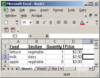
· Enter "Item" or "Food" in A1, “Section” in A2 and “Quantity Needed” in A3 and “Price” in A4, so that it looks like the following:

3. Enter items in rows 2 – 21.

· The “Section” is the section of the store in which the items would be found. For example, milk is found in the refrigerated section. CDs are in the music section. The section does not have to be very accurate – your best guess is fine. You can make up the price.

4. Format the price as currency.

· Highlight the first price. Hold the shift key down and highlight the last price, so that all the prices are highlighted. Choose format / cell / number and then choose currency.

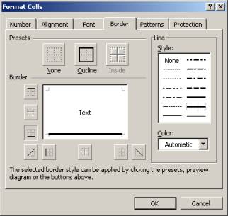
5. Format the 4 heading cells:

· Highlight the 4 heading cells. Choose Format / Cells from the menu. Choose the font tab. Choose a bold font style and single type of underline.

· Then, Choose the border cell and click on the heavy line picture and then click on the bottom only of the box. If you make a mistake and put a line where you don’t want it, just click on the line again to make it disappear.

· Your spreadsheet should now look like:

6. Make the column sizes fit with room to spare.

· Grab the bar between the A & B to drag it so that most food names fit.

· Repeat for section and quantity needed

7. Format the quantities and headings to be centered.

· Click on the number 1 to highlight the first row. Click on the center button.

· Click on the letter C to highlight the third column. Click on the center button.

8. Format all cells to be size 20 and wrap them all to fit.

· Click on the box between A & 1 to highlight the entire spreadsheet.

· Format / Cells and choose tab font and then size 20.

· Adjust the column sizes again if you want.

· Choose Format / Row / Autofit so that the minimum amount of space is taken by each row.

· It should now look like:

9. Total the quantity.

· Place your cursor below the last quantity. Press the sum button (which looks like a Greek E) and then press Enter.

· Format the page header and footer:

· Choose File / Page Setup and click the Header/Footer Key.

· Click on custom header.

· Enter “SHOPPING LIST” in the left box, your name in the middle.

· Click on the right box and then click on the date picture (which looks like a calendar)

· It will look like:

· Accept it with OK.

· Below the footer, just down arrow to choose the page 1 of x format.

10. Set the page orientation:

· Click the page tab (in page setup) and then choose the landscape button

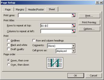
11. Set the headings:

· Click the sheet tab (in page setup) and then click on the box after “Rows to repeat at top”. Click on the row number 1 and then hit enter. Your Rows to Repeat at top box will then look like:

12. Accept the entire page setup by choosing OK until you see your spreadsheet again.