INVENTORY LIST STEPS For the
Simple List Sheet
Assignment: Create an inventory workbook with 4 sheets, and this document gives the instructions for the first sheet.
SHEET 1:
Step by Step Guide for SHEET I:
- Create a new Excel spreadsheet.
· Press Start / Program / Microsoft Excel (and you may need to first select Microsoft Office).
· Choose File / New / Blank Workbook to create an empty Excel spreadsheet.
· Choose Fiile / "save as" and then press the down arrow next to “save as type” to choose the Excel 97/2003 format.
· Enter your name as the spreadsheet name and save.
- Set the sheet label to "Simple List"
· Double click on the word "sheet1" at the bottom of the screen.
· Type "Simple List" and then enter.
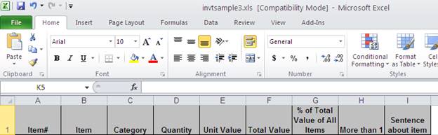
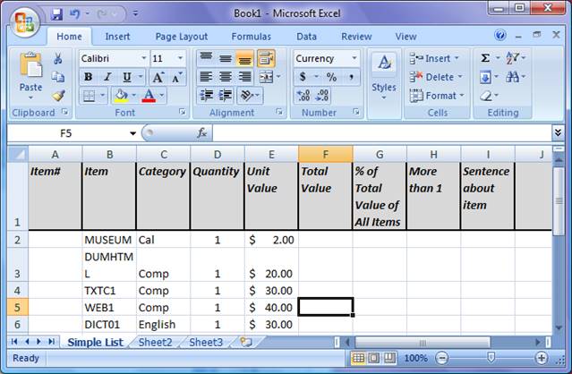
- Fill in the column headings: Enter : Column Headings: Item#, Item, Category, Quantity, Unit Value, Total Value, % of Total Value of All Items, More than 1, Sentence about item. (You can also add any other columns you want to add, such as a comment at the end.) - so that it looks like the following: (Tip: copy the columns names to word, convert text to table at commas, then copy from word to excel.)
- Enter items in rows 2 – 21.
· Only fill in Item, Category, Quantity and Unit Value. Everything else will be calculated.
· Item – Short item description.
· Category - A category code you create to group your items. At least two items must have the same category, and you need at least 2 categories.
· Quantity - only numbers (Add a comment or unit type column if you want to include a unit description.)
· Unit Value - the value of only one unit.You can just guess.
- Format the heading cells. Bold and italicize the words in the headings, and make the background color of the heading cells gray. Also, draw a thick border around the headings.
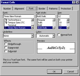
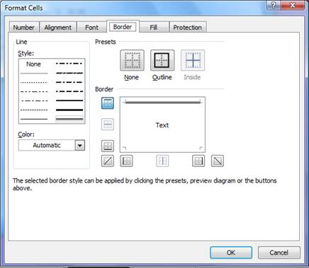
· Highlight all the heading cells in row 1, but do this by highlighting the individual cells, not the row. Choose Home tab, cells pane, format choice and then format cells option. Choose the font tab. Choose a bold italic font style.
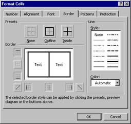
· Then, Choose the border tab and click on the heavy line picture and then click on the outline box and then the inside box, so all the lines in the "text" box are filled. If you make a mistake and put a line where you don't want it, just click on the line again to make it disappear.
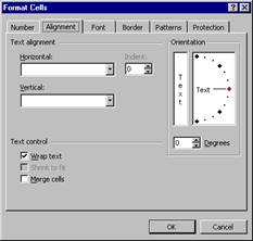
· Then, Choose the Alignment tab and click "wrap text" so the words don't bleed into other cells.
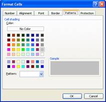
· Then, Choose the fill tab and click on any color you like to set the background color for the selected cells. If you make a mistake and put a background in the wrong cell, just choose the no color box.
·
· Your spreadsheet should now look like:
Note: If you want to create a macro so that you can format the heading this way whenever you want: see excelMacros.htm
- Format the values as currency.
· Highlight the first value. Hold the shift key down and highlight the last values, so that all the values are highlighted. Choose Home tab, cells pane, format choice and then format cells option. Then choose the number tab and then choose currency
- Format the quantities and headings to be centered.
· Click on the number 1 to highlight the first row. Click on the center button.
· Click on the letter D to highlight the quantity column. Click on the center button.
- Insert the Item Numbers using home tab / editing pane / fill (or down arrow) command.
- Enter 1 in A2 (the first item number)
- Highlight the first item number to the last item number. (Click item number and then hold the shift key down, scroll down to item 20 and click again to highlight all item numbers.)
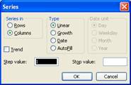
- Choose home tab, editing pane / fill (or down arrow) command and series option. (Note that the numbers increase by 1 because it steps by 1.)
- If you forget to enter the 1 in A2, it wont work.
- Make the column sizes what you want and wrap all the cells
- Grab the bar between the B & C to drag it so that most item names fit.
- Repeat for the other sections. (You may repeat this again as you add more to the spreadsheet.)
· Click on the box between A & 1 to highlight the entire spreadsheet.
· Choose Home tab, cells pane, format choice and then format cells option.and then hit the alignment tab.
· Hit the "wrap text" button until it is checked.
- Sort by Category, and then Item Number
· Highlight rows 2 - 21 by placing your cursor on the # 2 and then hold the shift key and click the number 21. You want all the rows selected, not just a few cells.
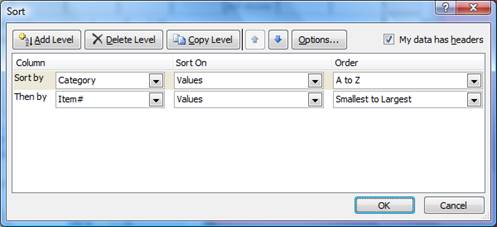
· Choose the data tab and then choose the sort command. Press the down arrow by the "sort by" box and choose the "category" label or column C. To then sort by item number within the category, click the "add level" button and then down arrow next to the second "sort by" box and choose either "item number" or Column 1. When you press okay, you will see all your items in a different order, but the same quantities should be next to them. If it is wrong, immediately choose Edit / Undo and try again. Be sure the entire rows are highlighted before you sort.
- Calculate the total value as quantity * unit value
- Place your cursor under the "total value" heading.
- Type = and then then click on the quantity in that row, and then type * and then click on the unit value in that row, and then press <ENTER>.
- Right click on that cell and choose copy.
- Highlight that cell and then hit shift and highlight the last total value cell so that all the total value cells are highlighted.
- Right click and choose paste.
- The total value of each items should be calculated.
- Total the quantity and total value columns with a double bar above them
· Place your cursor below the last quantity. On the formula tab, press the auto-sum button (which looks like a Greek E) and then press Enter. You will now have the total.
· Highlight that total cell
· Choose the home tab, cells pane, format command, format cells option.
· Choose borders
· Hit the double line tool
· Click on the line above the box so it looks like this:
· Click OK
· Copy that cell to the one under the last total value.
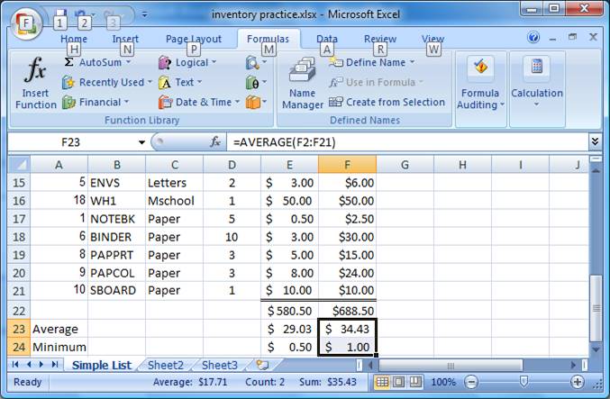
13. Calculate the average and minimum for quantity, unit value and total value:
- Below the items, skip one line and type Average and on the next line type Minimum to label the numbers you will calculate.
- Calculate the average quantity by placing your cursor in the cell under total quantity.
- Formula tab /function library pane / (maybe more functions) / statistical functions / AVERAGE
- Click on the little red spreadsheet box
- Highlight the first quantity through the last one and press ENTER twice.
- Calculate the minimum quantity by placing your cursor in the cell under average quantity.
- Formula tab /function library pane / (maybe more functions) / statistical functions / MINIMUM
- Click on the little red spreadsheet box
- Highlight the first quantity through the last one and press ENTER twice.
- Copy these functions to the unit value and total value columns by highlighting the two cells you just created and right click
- Choose copy
- Highlight the four cells under unit value and total value and right click and press paste.
- It should now look like this:
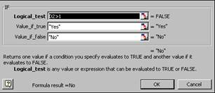
14. Under "More than 1", use an if statement to show "yes" if the quantity is more than one and "no" otherwise. (Do not just type in yes and no into the cells, and be sure at least one turns out to be yes and another no.)
- Click on the first cell under "More than 1".
- Formula tab /function library pane / (maybe more functions) / logical functions / IF
- The logical test is "Is the quantity more than 1?" This translates to is D2>1. Type "D2>1" in the logical test.
- Value if true = Yes
- Value if false = No
- Press <enter> twice.
- Copy this first cell to all the other rows with items.
- Change the quantity of an item to see the yes and no values change automatically.
15. Under "Sentence about item", create a concatenation of "I have " + quantity + " of " + long description.
- Click on the first cell under "Sentence about item"
- type = "I have " &
- click on the quantity
- type &
- type " of " &
- click on the item name
- press <enter>
- Copy this first cell to all the other rows with items.
- example: ="some words " & D2 & " other words " & E2 (and do not forget the equal aign). (This is for formatting only.)
- Change the quantity of an item to see the yes and no values change automatically.
16. Calculate the % of the total value of all items by dividing the total value for the row by the total value for all items. Use one formula for all the rows by properly setting the $ in the formula.
- Click on the first cell under "% of total value"
- type "=" (to tell Excel this will be a formula)
- click on the total value of that item (to put the excel address of the total cell into the formula you are working with)
- type / (to divide)
- click on the total value of ALL items (to divide by the total of all items)
- press <enter> (You should now have = F2/F<your last row>, which is the total value of one item divided by the total value of all items)
- in the formula bar, change the total value cell to have $ before the row and before the column. (You do this to make the total of all items remain the same when you copy the formula down.)
- press <enter>
- format / cell / number / percentage & ok
- Copy this first cell to all the other rows with items.
- example: A3/$Y$20 (This is for formatting only.)
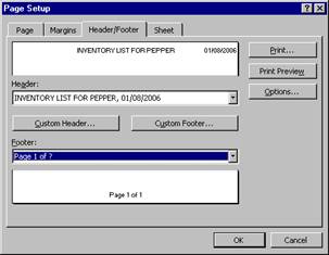
17. Format the page header and footer.
· On the page layout tab, find the page setup pane. Right after the words "page setup" is a little square dialog box. Click that box.
· Click the Header/Footer tab.
· Click on custom header.
· Enter "INVENTORY LIST FOR " and your name in the middle.
· Click on the right box and then click on the date picture (which looks like a calendar)
· It will look like:
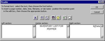
· Accept it with OK.
· Below the footer, just down arrow to choose the page 1 of ? format.
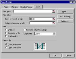
- Set the column headings:
· Click the sheet tab (in page setup) and then click on the box after "Rows to repeat at top". Click on the row number 1 and then hit enter. Your Rows to Repeat at top box will then look like:
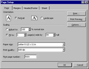
- Set the page to print only one page wide, so you don't have to tape two pages together.
- Click the Page tab
- Click the fit to button
- choose 1 page wide by 99 tall
- Set the Margins to 7 inches from the bottom
- Click the Margin tab
- Type 7 next to bottom
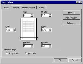
- Accept the entire page setup by choosing OK until you see your spreadsheet again.
- Make the Heading Cells ("Item", etc.) stay put when you scroll.
· First, be sure you are in normal view. Click the view tab and then normal.
· Click the row number 2 to highlight the entire row 2.
· Choose view tab/ freeze pane command.
· Scroll down to be sure that row one does not move.
- Print Preview by choosing the / Print Preview. It should print on 2 pages and have column headings at the top of each.
- Save your spreadsheet
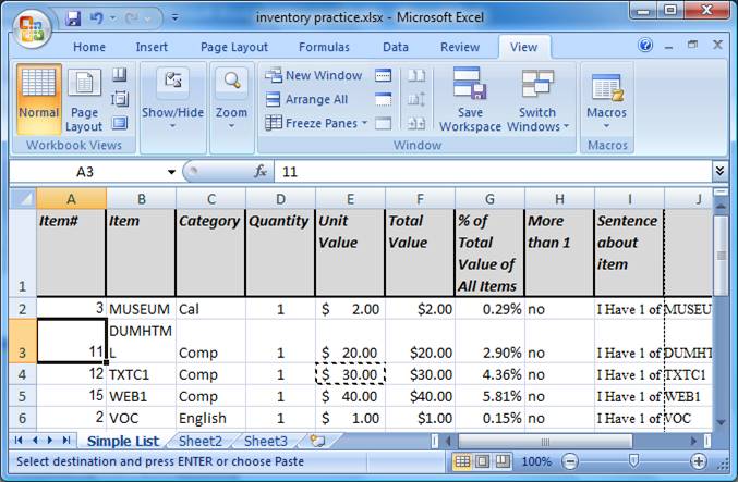
Your spreadsheet should look like this at the top (with your own items):
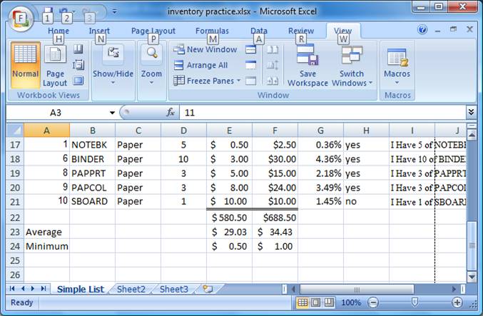
And like this at the bottom:
25. Now move on to Inventory Guide for Sheet #2 & 3 Written Instructions