INVENTORY LIST
Assignment: Create an inventory workbook with the following 3 sheets, and hand it in on the Excel project discussion board. Reply to project done and attach your completed spreadsheet. The spreadsheet must be first renamed to a file called your name.xls so that I can see from the filename that it is yours. If you prefer to create a list of items you might want to sell on Ebay, that would be okay.
SHEET 1:
· Heading: "INVENTORY LIST FOR " "<your name>" and the date
· Footer: page x of x
· Sheet tab label: simple list
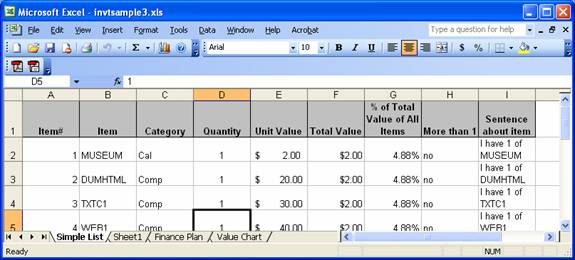
· Column Headings: Item#, Item, Category, Quantity, Unit Value, Total Value, % of Total Value of All Items, More than 1, Sentence about item. (You can also add any other columns you want to add, such as a comment at the end.)
· Bold and italicize the words in the headings. Also, draw a thick border around each heading and make the heading cells gray.
· List at least 20 items, but use formulas to create the following columns: Item#, total value, , % of Total Value of All Items, More than 1, Sentence about item.
· Remember that the quantity can only contain numbers
· Include at least two categories, and have at least two items in the same category.
· Center the quantity column.
· Format the values as currency.
· Sort by Category and then Item
· Calculate the total value as quantity times unit value
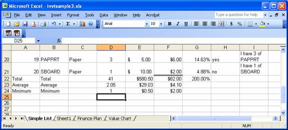
· Total the quantity and total value columns and put a double bar above the totals.
· Below the total, calculate the average quantity, unit value and total value
· Below the average, calculate the minimum quantity, unit value and total value
· Below the minimum, calculate the total number of lines in your inventory list using the COUNTA function.
· Under "More than 1", use an if statement to show "yes" if the quantity is more than one and "no" otherwise. (At least one item should have a quantity of 1 and at least one should have more than 1.)
· Use series fill to assign the item numbers.
· Calculate the % of the total value of all items by dividing the total value for the row by the total value for all items. Use one formula for all the rows by properly setting the $ in the formula.
· Under "Sentence about item", create a concatenation of "I have " + quantity + " of " + long description.
· Autofit the rows so that the height accomodates the contents.
· Set the Margin to 7 inches from the bottom, so that only about 17 lines will print on a page, and you will get two pages. The column headings should print on the second page as well.
· Freeze the column headings so they stay put when you scroll.
· Make your columns wide enough so that your row wouldn't fit on one page. (This means you will see a dotted vertical line through a row of words.)
· Set the page to print only one page wide, so you don't have to tape two pages together. (If the print is too small to read, wrap some columns so that the print isn't squeezed too small to read.)
Your first sheet should look like this at the top (with your own items):
And like this at the bottom:
optional: If you want to add a macro for creating headings, see here
SHEET2:
· Heading: "FINANCE PLAN FOR " <your name>"
· Footer: Date, filename and page number. (Use a custom footer)
· Sheet label: Finance Plan
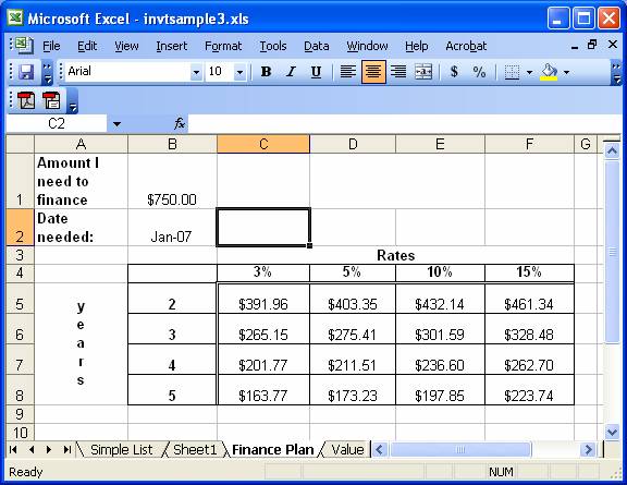
· On the first line, show "Amount I needed to Finance" and in the cell next to it, show any amount (other than 750) formatted as currency.
· Wrap the "Amount I needed to Finance" cell so it appears on 2 lines.
· On the second line, show "Date Needed" and in the cell next to it, show the date January 2, of this year.
· Format the date so it shows as "the month abbreviated-the year" (ex: Jan-07)
· Merge C3 to F3 and write "Rates" and bold and center it.
· Merge A5 to A8 and write "Years" and bold and center that.
· Turn "Years" so it prints vertically.
· In C4-F4, enter the rates 1%, 5%, 10% and 15%
· In B5-B8, enter the years 1, 3, 4 and 5
· Calculate the payment amount for the loan needed for each interest rate/ year combination. (Loans are compounded annually.) This should be done be creating the formula once, and copying it to all the other cells in the grid. The payment should be formatted as currency. Do not enter the formula more than once.
· Change the amount you need and see all the numbers in the grid change.
· Bold all labels.
· Center everything in columns B through F.
· Put gridlines around the years and rates and all the payments. Below the year and rate labels, place a double line. It should look something like the following:
SHEET 3:
· Heading: "VALUE CHART FOR " <your name>"
· Footer: Date, filename and page number. (Use a custom footer)
· Sheet label: Charts
· Using the chart wizard on the finance sheet, create a simple chart by just highlighting the entire table from A4 to F8. Use the chart wizard and just take all the defaults. Your chart should look something like:
· Using the chart wizard on sheet 1, create a column chart with the following:
- Title: Comparison of total units and values
- y axis label - "value"
- x axis label - "item number", with the numbers being taken from column A
- Series 1 - Unit Value, with the label being taken from row 1
- Series 2 - Total Value, with the label being taken from row 1
- The chart should look something like:
SHEET 4:
This sheet should contain any spreadsheet that is useful to you in some way and looks nice when printed. This sheet is unrelated to the inventory sheets. It is just in the same workbook. It could help you track something for your job, a club or a hobby. It could be a game or help you solve a puzzle. (A suduko excel spreadsheet could check that all the numbers totaled 9, and maybe be even more help than that.) It could even be a sheet you used to help you in another class, perhaps to help you create a graph that you copied into a report.