STEP BY STEP GUIDE FOR INVENTORY SHEET #2 & #3 Excel 2011 – to current

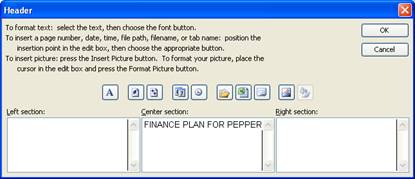
1. Heading: “FINANCE PLAN FOR “ <your name>“

o First open your inventory workbook.

o Then, click on the tab sheet2 to get to the second sheet.

o On the file menu, choose the page setup option. Then click on the header/footer tab and then click on the custom header button

o The header should be empty. If it has a heading already, you are probably not in sheet 2, so go back and click the sheet 2 tab first.

o Type Purchase Plan for “<your name>“ (not Pepper) like below:

o Click OK

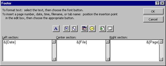
2. Footer: Date, filename and page number.

• Click the custom footer button
• Click in the left section and then click the calendar button
• Click on the center section and then click the x over a paper button
• Click the right section and then click the number sign button.
• Click OK

3. Sheet label: Finance Plan

• Double click the sheet tab and type Finance Plan

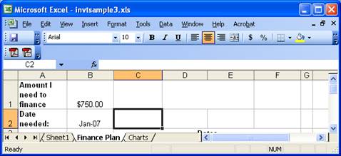
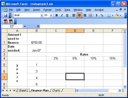
4. On the first line, show “ Amount I need to finance” and in the cell next to it, show any amount formatted as currency. (Do not use 750.)

• Click in cell A1 and type “ Amount I need to finance “.
• Click in cell B1 and enter the amount of money you want to have to borrow.
• Click on the $ button in the home tab in the Number pane at the top of the screen or right click (or command click) on the cell and choose format cells / number / currency.

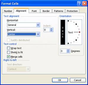
5. Wrap the “Amount I needed to Finance” cell so it appears on 2 lines.

• Highlight A1 and right click to choose format cells.
• Choose the alignment tab.
• Click the wrap box until it is checked and then choose ok.
• See that the words show on two lines now and don’t cross the cell border.

6. On the second line, show “Date Needed” and in the cell next to it, show the date January 2, of this year. Format the date so it shows as “the month abbreviated-the year” (ex: Jan-11)

• Click in cell A2 and enter “Date Needed”.
• Click in the cell next to it (B2) and enter 1/2 and then press <Enter>.
• Right click to choose format cells, then the number tab and then choose the date format that matches Jan-08, with 08 being the year, not the day.
• Hit <Enter>.
• It should now look like:

7. Merge C3 to F3 and write “Rates” and bold and center it.

• Highlight C3 to F3
• Right click to choose format cells and choose the alignment tab.
• Keep clicking the merge cells box until it is checked.
• Hit <Enter> to accept it.
• Type “Rates”.
• Click the bold and center buttons on the home tab and font and alignment panes.

8. Merge A5 to A8 and write “Years” and bold and center that. Turn “Years” so it prints vertically.

• Highlight A5 to A8
• Right click to choose format cells and choose the alignment tab.
• Keep clicking the merge cells box until it is checked.
• Then, to make it print vertically, type -90 in the orientation box (next to the word degrees), and then highlight the box that says “text” and see that it is still at 0 degrees (which means the letters themselves wont be turned).
• Under vertical alignment, choose center so that the “Years” will not be at the bottom.
• Hit <Enter> to accept it.
• Type “Years”.
• Click the bold and center buttons
• Make rows 5-8 a little bigger to fit “years” by Highlighting the row numbers 5-8 and then dragging the line between 5 & 6 to make it a bit bigger. All highlighted rows will become bigger.

9. In C4-F4, enter the rates 1%, 5%, 10% and 15% and in B5-B8, enter the years 1, 3, 4 and 5.

• Just enter 1% in C4, 5% in D4, 10% in E4 and 15% in F4.
• Also enter 1 in B5, 3 in B6, 4 in B7 and 5 in B8.
• It should now look like this:

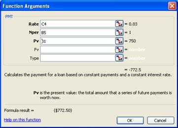
10. Calculate the payment amount for the loan needed for each interest rate/ year combination. (Loans are compounded annually.) This should be done be creating the formula once, and copying it to all the other cells in the grid. The payment should be formatted as currency. Do not enter the formula more than once.

• In cell C5, choose the formula tab and then insert function.
• Select the category financial.
• Choose the function PMT
• Press <Enter>
• Double click inside the parentheses, and then:
1. click on the rate in C4 and then type a comma
2. now you see Nper (number of periods) highlighted, so click the year 1 and then type a comman
3. now you see Pv (present value – the amount you want to borrow) highlighted, so hit the amount you want to borrow in B1
4. You can now click fx to see the formula in the formula builder.
• Press <Enter> again to accept the formula.
• Press the $ button on the home tab to format this number as a currency. (If you want it to be a positive number, you would need to multiply the amount borrowed by -1.)
• See the payment amount. It should be just a little more than the amount you are borrowing because the interest is low and you are only making 1 payment.

11. Adjust the formula so it can be copied to the other cells in the table.

• Highlight cell C5 to see the PMT formula in the formula bar.

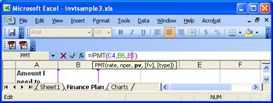
• Put a $ before any row or column you want to stay put when you copy the cell. Leave the $ out when you want excel to move the row or column when you copy. For the rate, you will want to keep the row the same and let the column move. For the year, the column will stay the same and the row will move. Make your best guess at where the $ signs belong. (ex: C$5 to hold the row as 5 or $C$5 to hold the cell as C5 or $C5 to hold the column as C). Press <Enter> when you are done with your first guess.
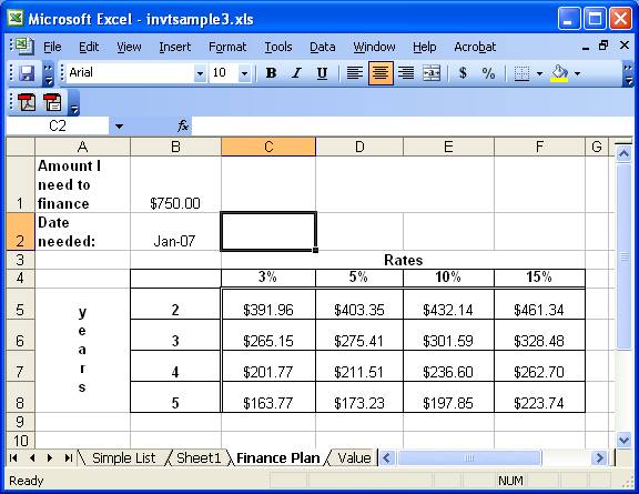
• Copy C5 to all the cells from C5 to F8.
• Format all these cells as currency by pressing the $ button.
• Verify it is correct by asking:
• Are all the 1 year loans a little bigger as the rate increases?
• Are 1% loans smaller as the number of years increases?
• If the answers are yes, you are done. If not, go back to C5 and change the $ signs an repeat the copy until it is correct.

• Change the amount of money you want to borrow and see all the numbers in the grid change.
• (Extra credit – You have now calculated the payment each year if the loans were accrued annually. Change the formula to calculate a monthly accrual, and write the word MONHLY in D1.)

12. Bold all labels.

• Highlight row 4 by clicking on the number 4
• Press the B button on the home tab
• Highlight column A by pressing on the A letter
• Press the B button on the home tab
• Highlight B5-B8
• Press the B button on the home tab

13. Center everything in columns B through F.

• Highlight columns B through F by clicking on the B and then holding until you reach the F.
• Click the center button on the home tab.

14. Put gridlines around the years and rates and all the payments. Below the year and rate labels, place a double line.

• Highlight B4 to F8
• Right click to choose Format Cells and click the border tab
• Choose the outside and inside
• Hit <Enter>
• Highlight just the interest rate labels (C4-F4)
• Right click to choose Format cells /border
• Choose the double line border
• Click only on the bottom of the cell.
• Hit <Enter>
• Highlight just the year labels (B5-B8)
• Right click to choose Format cells /border
• Choose the double line border
• Click only on the right of the cell
• Hit <Enter>
• It should look something like the following:

15. Set it to print landscape so that it prints on the page the long way

· Choose the layout tab, orientation command and then click on the landscape box.

16. Start on Sheet 3 by clicking on the Sheet 3 tab, or home tab, insert command, insert worksheet option.

17. Heading: “VALUE CHART FOR “ <your name>“

o First open your inventory workbook.

o Then, click on the tab sheet3 to get to the second sheet.

o On the file menu, choose Page Setup and click on the header/footer tab and then click on the custom header button

o The header should be empty. If it has a heading already, you are probably not in sheet 3 so go back and click the sheet 3 tab first.

o Type Value Chart for “<your name>“:

o Click OK

18. Footer: Date, filename and page number.

• Click the custom footer button
• Click in the left section and then click the calendar button
• Click on the center section and then click the x over a paper button
• Click the right section and then click the number sign button.

• Click OK

19. Sheet label: Charts

• Double click the sheet tab and type Charts

20. Using the chart wizard on the finance chart, create a chart of the possible payments:

• Go back to sheet 2 (your finance plan sheet) and highlight from A4 to F8 (so that the words “rates” and “years” are both highlighted.
• Choose the chart tab / all charts command and choose a 3-D column chart and press <Enter>. It will create a chart for you that looks something like the one below (with different numbers):

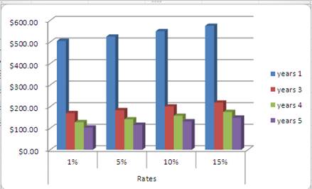
• Move your chart to the chart sheet by highlighting then entire chart box (not just a portion) and right clicking to choose cut. Then right click on your chart sheet and choose paste.

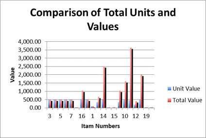
21. Using the chart wizard on sheet 1, create a column chart with the following:

• Title: Comparison of total units and values
• y axis label - “value”
• x axis label - “items”, with the numbers being taken from column A
• Series 1 - Unit Value, with the label being taken from row 1
• Series 2 - Total Value, with the label being taken from row 1
• The chart should look something like:

Steps to create the chart:

• In Sheet 1, highlight the unit value starting at E2, through the last total value. (So you should have 2 columns highlighted.)
• Choose the chart tab and a the all charts icon and choose a 3d chart style from the menu.
• It will create a chart and the design tab will display. Choose the move chart command on the design tab in the location pane. Change to “object in” and down arrow to choose “charts”. (If the design tab does not appear, Double click on the chart so the design tab appears.)
• If the names unit value and total value do not appear on your chart:
• Set the series names: Choose select data in the data tab, highlight “series 1” and then choose edit. Next to series name, type “unit value”. Hit <Enter>.
• Highlight the series2 label and hit edit. Then type “Total value” and hit <Enter>.

• Set the x axis labels by clicking on the design tab (which you only see when you click on the chart), select data command, and then see x axis labels. Click the spreadsheet button and Then, click on the simple list sheet, and then highlight the first item number through the last item number and hit <enter> and then hit <OK> repeatedly until you see the graph again.

• To add a title: on the chart layout tab, choose the chart title. Then double click the chart title and change it to: “Comparison of total units and values”;
• To add axis labels, on the chart layout tab, choose the chart axis labels icon and set a horizontal and vertical label. Then change the bottom axis title to “Item Numbers” and change the side axis to “value”.

• You will need to highlight the whole chart (not a piece) and move it lower on the sheet so it doesn’t cover up the other chart.