INVENTORY LIST

Assignment: Add the three sheets specified to your inventory sheet from last week. .

To hand it in: Upload one workbook with all 4 sheets to moodle.

How to Start:

• If you prefer to dive right in: Read the requirements below and create your sheet.
• If you prefer a movie or written instructions guiding you along: 
• use the step by step instructions for sheets 2-3
• use these step by step instructions for sheet #4.
• The first row has the written instructions and the rest contain movies.

SHEET2:

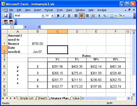
· Heading: "FINANCE PLAN FOR " <your name>"

· Footer: Date, filename and page number. (Use a custom footer)

· Sheet label: Finance Plan

· On the first line, show "Amount I needed to Finance" and in the cell next to it, show any amount (other than 750) formatted as currency.

· Wrap the "Amount I needed to Finance" cell so it appears on 2 lines.

· On the second line, show "Date Needed" and in the cell next to it, show the date January 2, of this year.

· Format the date so it shows as "the month abbreviated-the year" (ex: Jan-07)

· Merge C3 to F3 and write "Rates" and bold and center it.

· Merge A5 to A8 and write "Years" and bold and center that.

· Turn "Years" so it prints vertically.

· In C4-F4, enter the rates 1%, 5%, 10% and 15%

· In B5-B8, enter the years 1, 3, 4 and 5

· Calculate the payment amount for the loan needed for each interest rate/ year combination. (Loans are compounded annually.) This should be done be creating the formula once, and copying it to all the other cells in the grid. The payment should be formatted as currency. Do not enter the formula more than once.

· Change the amount you need and see all the numbers in the grid change.

· Bold all labels.

· Center everything in columns B through F.

· Put gridlines around the years and rates and all the payments. Below the year and rate labels, place a double line. It should look something like the following:

SHEET 3:

· Heading: "VALUE CHART FOR " <your name>"

· Footer: Date, filename and page number. (Use a custom footer)

· Sheet label: Charts

· Using the chart wizard on the finance sheet, create a simple chart by just highlighting the entire table from A4 to F8. Use the chart wizard and just take all the defaults. Your chart should look something like:

· Using the chart wizard on sheet 1, create a column chart with the following:

• Title: Comparison of total units and values
• y axis label - "value"
• x axis label - "item number", with the numbers being taken from column A
• Series 1 - Unit Value, with the label being taken from row 1
• Series 2 - Total Value, with the label being taken from row 1
• The chart should look something like:

SHEET 4:

This sheet should contain any spreadsheet that is useful to you in some way and looks nice when printed. This sheet is unrelated to the inventory sheets. It is just in the same workbook. It could help you track something for your job, a club or a hobby. It could be a game or help you solve a puzzle. (A suduko excel spreadsheet could check that all the numbers totaled 9, and maybe be even more help than that.) It could even be a sheet you used to help you in another class, perhaps to help you create a graph that you copied into a report.