(Note: If you are on a mac, you might need to press Control while you click
your mouse in order to get a “right click” menu.)
- Copy the data from the web site into your spreadsheet:
- First copy the rows of
information on this page to excel.
- Start at the "Rk" heading and copy down through the last
player on this page. Right click and choose copy.
- Then, start / program
/ openoffice / spreadsheet and then
“right click” on A1 and choose paste.
- Remove hyperlinks by
highlighting the entire sheet (click between
A and 1 to highlight the entire sheet) and then choose format / default
formatting to remove the hyperlinks.
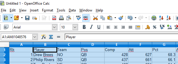
- Your sheet should look
like the following (with different information but the same headings):

- If you do not end up with a spreadsheet that looks like
the one above: just download this starter spreadsheet instead:
- Right click on starter sheet to see the context menu.
- choose "save target as"
- choose "open"
- You can highlight an
entire spreadsheet by clicking on the upper right square
- You can remove
hyperlinks by using format / default formatting
- Different browsers
handle copying tables differently
Step 2: Formatting: Watch Video Instructions
- Put a light border around all cells with something in them (highlight all cells with data by
clicking ctrl end [ or FN ^ ->] and then use the scroll bars to get
back to the top and hold shift and then click A1. Then right click to
format cells / border / and click on a thin line and then click on outline
and inside. )
- Wrap cells so you can see the entire player name: (format cells / alignment / make the
“wrap text automatically” checkmark solid and not gray)
- Add a header saying Runningback Stats and
a footer with page number (Format / Page and then
header tab / then edit / and then in custom header type "Runningback
stats" and press ok and then click the footer tab and then edit and
then down arrow on the footer and choose a page number format and press ok
twice)
- Change it to print landscape instead of portrait (longways): (Format / Page and then choose the page
tab and click landscape)
- Print preview and see how it would print. (file / page preview and scroll down to
see next pages then close preview.
- Change to print column headings at the top of each page: (Format / Print Ranges / Edit and then
down arrow under “rows to repeat” to change it to “user defined” and then
type $1 to indicate row 1 should repeat. Then choose OK)

- File / Page preview to see it shows now prints column headings on
every page. But see that you would have to tape together 2 pages to
get all columns across. Close Preview.
- Make it smush to one page wide – without adjusting the
column size: (File / Page / page,
sheet, down arrow below “scaling mode” and choose “fit print ranges to
width/ height” and then set width to 1 and height to 99. ) It will never stretch to 99 pages, but will squeeze to 1 wide.
- File / Page preview to see you no longer have the extra pages with the
small columns and also verify it is at least 2
pages. If it is only one page, you might have chosen 1 high. Close Preview.
- Try scrolling around the spreadsheet to see some
problems:
- Scroll down and see headings move.
- Scroll across and lose player names.
- Change to show headings on screen as you scroll down
and across. ( Click once on C2 and
then window / freeze) It
will freeze to the left and above the highlighted cell.
- After you freeze, Scroll down
and across and see the labels stay still
Step 3: Concatenate Text: Watch Video Instructions (Excel is the same for this so you
can follow this video in your open office spreadsheet.)
Step 4: Calculating simple references: Watch Video Instructions
- Add a column to show the sum of each players 20+ and 40+ (Insert a column
by Highlighting all of column T by clicking the T and then right
click to choose insert. Type = in T2 and then
click on R2 and then type + and then click on S2 and then press Enter.
Right click to copy T2 and then highlight all the empty cells
in column T and right click to paste)
- Sum the total yards
column. (Put your cursor
below the last yard - J52 - and type "=SUM("
and then highlight all the numbers above and then press Enter)
- Find the average of the yards ( Put your cursor
below the total - J53 - and hit
insert function on the left - and choose average - then highlight
all but the total cell.)
- Find the maximum values in the yards
column. (Repeat above while moving down one row each time, but select
the max function instead)
- Find the standard deviation of the yards. (Just repeat
above but select the stdev function instead. -
Standard deviation is a measure of how spread out these numbers
are - For more details on the
meaning of standard deviation, read this, and notice how easy Excel or
Open Office Calc makes complex formulas.)
Step 5: Calculating using absolute reference: Watch Video Instructions (Excel is the same for this so you
can follow this video in your open office spreadsheet.)
- Add a column to show the % of total yards for each player.
(Insert a column by highlighting the K column and right click
to insert. In K2, type = and then click on J2 and then "/" and
then click on the total J52 and press enter. Try to copy it down and find
that it keeps moving the J52. Back in K2, change J52 to J$52 and try the
copy again.)
Step 6: Sort Watch Video Instructions
- Sort by player name (and make sure you do not change their stats).
(Highlight all the rows you want to sort, which is every
row. You can highlight the entire sheet by clicking the box
between A and 1. Then Data / Sort and choose the options tab and
click “range contains column labels” to tell it not to sort your heading
row and then click the sort criteria tab and then down arrow under
"sort by" (or column) and choose player and enter.)
- Sort again by player within team. (Data /
Sort and then down arrow under "sort by" (or column) and
choose team. Then down arrow under
“then by” and
choose player name. )
Step 7: If Watch Video Instructions
- Add a column with a “yes” if total yards > 1000 (Insert a
column by highlighting the K column, right clicking and inserting. Click
on K2 and then insert / function. Chose category logical and
then double click "If" and see 3
boxes. In the logical test, type "J2> 1000". Next to value if true, type
"yes". Next to value if false, type "no". Remember to
include the quotes on yes and no. Copy that formula down.
) Change one yard to be less than 1000 and another to be
more than 1000 and see how the result changes in column K.

