Excel
homework - Address List
Make an address list Overview (A step by step
guide follows)
- include
the following columns: first name, last name, address, city, state, zip,
phone, type, full name
- note:
type = F (for family), W (for work), S (for school), X (for friend)
- make
each column a reasonable size for the data
- make
at least one entry in the address column wrap
- sort
first by type and then by last name.
- Put
your name in the header
- Have
the title "Address List" centered across all the columns (and
have it be in the worksheet, not header)
- Put
the page number, date and filename in the footer
- align
everything to the left, even the zip code
- create
the full name automatically column using the first and last name columns.
- fit
to 1 page wide to print it.
- At
the bottom, put a count of the number of people, using the count function
- For
extra credit, show a count of each type.
Print out the spreadsheet and
hand it in.
Step by Step Guide:
- Create
a new Excel spreadsheet.
Press Start /
Program / Microsoft Excel (and you may need to first select Microsoft Office).
Choose File / New /
Workbook to create an empty Excel spreadsheet.
- Fill
in the column headings:
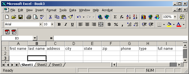
Enter "First
Name" in A1, and continue through to "Full Name", so that it
looks like the following:
- Fill
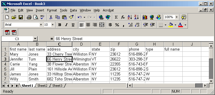
in information for 10 people you know. In the type column, enter F for
family, W for work, S for school, or X for friend .
Leave the full name column blank. It should look like the following, but
have your names listed:
- Change
the column sizes so that every column shows the full information, except
for the address column.
Put your cursor in
the first row (the one with "A" and "B" labelled),
and position your cursor on the line between the two letters. Your cursor will
become a line. Left click the mouse and drag to the desired column size.
- Wrap
the address column.
Highlight the
address column by clicking the label "C". Then
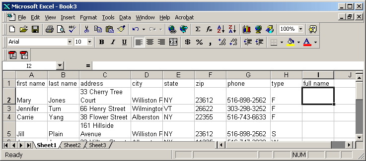
Format / Format cells / Alignment / Wrap text. (At least one of your
addresses should actually wrap to two lines. If they are all too short, enter a
longer description.) It should now look like this:
- Sort
by type and then by last name.
Highlight all the rows
of names by clicking the number "2" in the row label and then
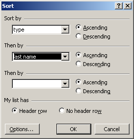
dragging your mouse down to the last row of names. Then, choose Data / Sort and
then choose type (or F) in "Sort by" and last name (or B) in
"Then by". Then, press OK to see it sort all of the same type
together, and then the last names in order.
- Put
your name in the header, and put the page number, date and filename in the
footer
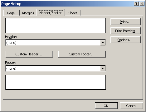
Choose File / Page
Setup and then the header footer tab and then custom header. Enter your name in
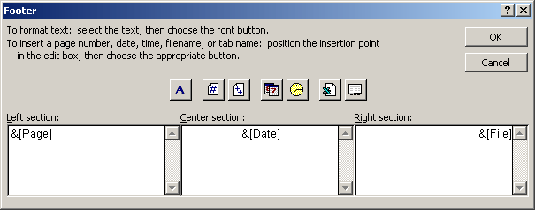
the center section. Then, choose okay. Then set the footer by choosing the
custom footer button. Pull the page number to the left. Pull the date picture
to the middle and pull the filename picture (X) to the right.
- Fit
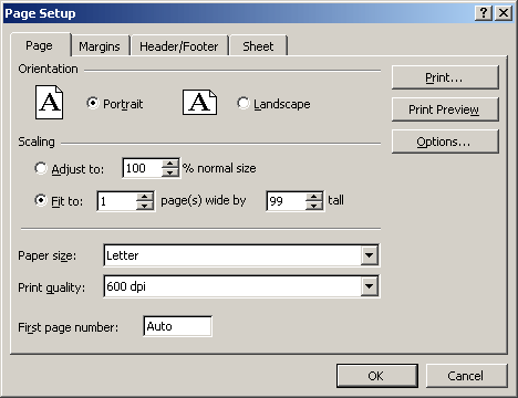
the page to 1 wide, but don’t restrict the number of pages printed.
Choose file / page
setup and click fit to. Then, change the pages tall to 99 (by typing in 99).
- Fit
the page to 1 wide, but don’t restrict the number of pages printed.
Choose file / page
setup and click fit to. Then, change the pages tall to 99 (by typing in 99).
- Have
the title "Address List" centered across all the columns (and
have it be in the worksheet, not header)
Insert 2 rows above
the titles. Highlight the row label 1, and then choose Insert / Rows. Repeat
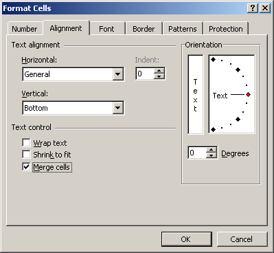
Insert / Rows. Then, type "Address List" in A1. Then, highlight A1 –
I1, (and do not highlight the entire row), and then choose format / cells /
alignment / and check the merge box. Click okay. Then click the center box to
center the words "Address List". The merge box is on the following
screen:
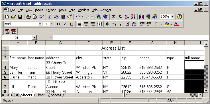
- Align
everything to the left, even the zip code
Highlight rows 3 –
the end of your list and hit the left align button. Your spreadsheet should now
look like:
- Create
the full name automatically column using the first and last name columns.
In I4, enter
"=" and then press on the first name in that row. Then enter &
" " & to add a space. Then, press on the last name in that row.
Press enter and see the first and last name in I4. The formula should look like
=A4& " " &B4. Copy that formula to all the other full name
spaces. (Highlight I4 and press Edit / copy and then highlight the empty full
name cells and press edit / paste.
- At
the bottom, put a count of the number of people, using the count function.
Put your cursor
under your Zip code column. Then, choose the menu option Insert and then choose
function (or you could hit the FX function box). Then, find the count function and double click
on it. (You can find the count function by first choosing the category “ALL”
and then scrolling down to “COUNT”. You
should see a box like the following appear:
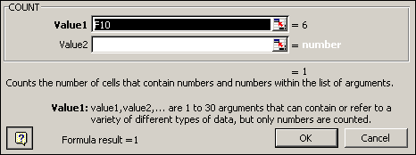
Hit the little
spreadsheet box next to value 1. It will bring up a box like this:
![]()
Put your cursor on
the first zip code (F4) and drag it down to the last zip code and then press
<ENTER> twice. You should now have this formula: =COUNT(G4:G9).
You should see the number of names you have as the count. Label it by entering
the word "Count" next to your count. Highlight that word.
- For
extra credit, show a count of each type.
You want it to look
like this:
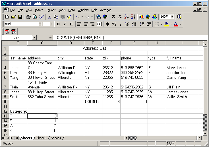
14. If you can, create a table listing the number of
names for each type. You DO NOT HAVE TO DO THIS.
Enter the word
"Category" in column A under your last row entered.
Enter the word
"Count" next to that value.
Under Category,
enter the types F, X, W and S as you see in the example above.
Next to F, enter
"=COUNTIF" and press the "=" sign next to the formula bar.
You will see the following:

Hit the spreadsheet
button next to the "Range" and then highlight all the type values in
your list. Then press Enter.
Hit the spreadsheet
button next to the "Criteria" and then highlight the category
"F" right under the word "Category."
Hit Enter twice to
accept it. You will see the formula similar to: =COUNTIF(H4:H9,B13)
Now, you want to
change that formula to tell excel that you don’t want it to change the range of
type values when you copy it to other cells. To do that,
place a "$" before each row and column in the range. You will
now have a formula of: =COUNTIF($H$4:$H$9,B13). You
can then copy that formula to the three rows below it.