Steps to perform Internet Data Analysis: Pivot and Lookup

Overview:

Practice pivot tables and lookup commands so that you can understand what power they have to save you work, and so that you know it can be easy to use. I am not expecting you to remember the mechanics, but rather to know how these features can help you.

· Why pivot tables: Pivot tables are very useful for quickly categorizing a list and getting totals. It is quick and powerful. You do need nice column headings and no merged cells, which can be tricky.

· Why Lookup: There will be times in your life that you are looking at 2 spreadsheets that you have to compare or match up in some way. Many people solve that manually, with lots of typing. Knowing the VLOOKUP commands power will help you match up columns from spreadsheets quickly.

Requirements:

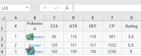
· 2 sheets of tables that are copied from the internet and have 1 column in common. I suggest 2 tables in these links:

https://pokemongo.gamepress.gg/pokemon-list

http://www.dltk-kids.com/pokemon/pokelist.htm

· One pivot table with some row categories and some values calculated inside the pivot chart.

· Use of VLOOKUP on sheet 1 to lookup values in another sheet based upon matching cells.

Movies:

· Excel Movie

o Overview

o Step 1

o Step 2 - End

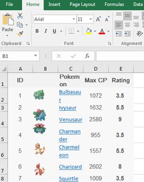
· Open Office Movie for entire project Please note this movie has one problem: the pokemon site added 3 columns. To adjust for this, after copying the columns to Excel, please delete the columns C - E (STA, ATK and DEF) and then rename CP (in cell F1) to Max CP. If you have trouble copying from the website, look at the Excel Step 1 video.

Detailed Instructions :

STEP 1: Copy table of information from the internet into Sheet 1 (I am recommending a particular table found on the internet but you can use any that you like on any subject.)

· You can go to any internet page that has a table of numbers. https://pokemongo.gamepress.gg/pokemon-list

· Copy the table by highlighting the top left cell (in this case hold your cursor down a centimeter left of the “ID” heading and then scrolling to the bottom right of the table and then hold SHIFT and click next to the bottom right cell.

· Hit control (or cmd on mac) and C at the same time to copy (or right click and choose copy)

· Open an Excel workbook.

· Right click in cell a1 and hit paste. And see the table in Excel.

o If it did not turn into columns:

§ For excel: highlight all pasted information and click on the data tab and then text to columns

§ For open office: try again with the google chrome browser

o Do note that the pictures copied but wont be very helpful to us.

· Your spreadsheet now has columns of information, including at least one with numbers.

· In order to match the movie, please delete the columns C-E and rename CP to Max CP. The site added 3 more columns recently, and these are not in the videos.

You are welcome to ignore the pictures as they will not matter, but if they bother you, hit F5 to get the “go to” dialog, and then click on the button named special at the bottom of the window and then choose objects. That will highlight all the objects and then you can just hit the delete button. Remember it is okay for the pictures to hang out and cover the words.

STEP 2: Place a pivot table of sheet #1's information into sheet #2. Show some analysis that either counts values or sums numbers.

First add another sheet by clicking on the plus sign at the bottom of your worksheet. You may need to maximize your window to see that plus sign:

Then make sure all your columns have good short names. There can be no special characters so change all your headings:

See how there are no special characters like % or = or ( in those names. Note that in our example we will be ignoring the pictures because they are not really attached to a cell, but we needed every column to have a name.

Highlight the entire sheet by choosing the cell between A and 1:

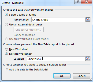
Step 2 A – For Excel : Actually creating the pivot table is different for Excel and Open Office, so follow the Step 2 A for Open Office if you use that.

Then choose insert tab, pivot table and click on "existing worksheet" and then click the button next to location and navigate to cell A3 in your new sheet. :

Then press OK to create your pivot table, which will have fields on the right side and the pivot table in A3:

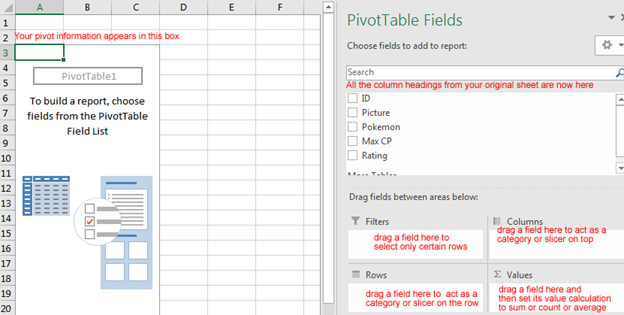
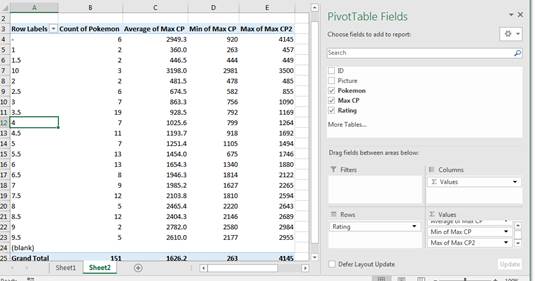
Now you can create a pivot table by dragging from the fields into the filter, columns, rows and values boxes: (We will slice rows by Rating and get a count of pokemon and their average, min and max MAX CP)

· Drag rating to the rows box.

· Drag ‘Pokemon’ to the values box (and it will automatically try to count them, which is good). You now know that there are 19 pokemon in the list with 3.5 rating.

· Drag ‘ Max CP’ to the values box and then click the down arrow next to “count of max cp” and choose “value settings” and change to Average.

· Drag ‘Max CP’ once more to the same values box and this time change its value setting to Minimum.

· Drag ‘Max CP’ yet again and this time change its value setting to Maximum.

· Format the average to have only 1 decimal: Highlight the average MAX CP columns and format / cells / number / set 1 decimal place.

· Your pivot table should look something like this now, with row categories and some calculations in each cross section:

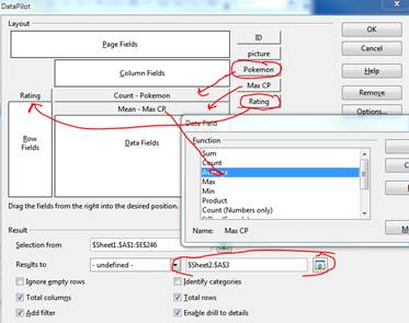
STEP 2A – For open office (If you use Excel, skip down now to STEP 3)

· Choose data menu, then data pilot option and then start, and then enter to accept the current selection, and then see a pivot grid.

· Drag the rating button onto the row field section of the pivot grid.

· Drag the pokemon and max cp buttons onto the data fields

· Then double click the sum- pokemon and change it to count and hit ok

· Double click the max cp and change it to average and hit ok

o (In open office, it doesn’t easily allow max cp to be used in 3 measures, so we will just look at average Max CP.)

· Click on the more button and then click on the results to spreadsheet icon and then click on sheet 2 and then a3 cell and then press enter. (If you miss this, your pivot will be below your table.)

· Then hit okay to accept the pivot grid which should look like the screen below. Then you can click on sheet 2 to see your pivot.

You will see a pivot table that looks like the one below: It does give you the calculations but not as nicely as in Excel. You can see that you have only 2 pokemon in your list at 1.5 rating and their average max CP is 446.

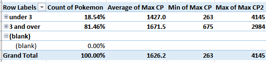
STEP 3: Play with the pivot table a little bit to drill down, group and show percentages.

· Drill down : Double click on a number in your pivot table and see it open a new sheet with only those pokemon that are represented in the cell you clicked.

· Percentages (cannot be done in open office so skip if using open office): Show all counts as percentages of the total column. Right click on a number in our pivot table and choose show value as and then choose % of total column.

· Optional: Group all ratings under 3 in 1 category (cannot be easily done in open office so skip this if using open office; You can also skip this if you find that your ratings are not sorting properly): Highlight ratings – to 2.5 and then right click and choose group. Click the minus sign by the group. See the statistics group correctly. Just write over the group name to rename it ‘Under 3’

o Repeat this process for all the other ratings (except blank) , naming them ‘3 and over’

o See how you can toggle with the plus sign.

STEP 4. In Sheet #1, write 3 values from one column in a new sheet. Use the HLOOKUP or VLOOKUP function to find values from the new sheet.

· Go to http://www.dltk-kids.com/pokemon/pokelist.htm

· Copy the entire tale including the column headings just as you did in step 1.

· Click on the + in the spreadsheet to create a new sheet and past in the pokemon type table.

o Format the text as Arial 11 so it looks nicer.

o If it were not sorted, you would have needed to sort by pokemon name.

· Name the sheet ‘types’

· Click back to the first sheet, the one you used for your pivot data.

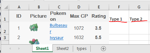
· Add a column for type 1 and another for type 2:

· Do the lookup in the first row that has a value you want to lookup.

o For Excel: From the formula ribbon, choose Insert function, type vlookup, and double click it.

o For Open Office: Insert menu / function option/ and then down arrow until you find VLOOKUP and double click it and hit Next. Your 4 lookup parts will mean the same thing but have different labels from the picture below.

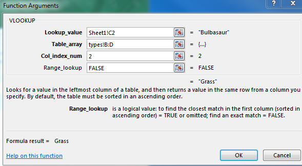
· Your lookup value should be the value that will match to the lookup table, so in this example, click c2. The table is the type table, so click on the types table and then highlight columns b, c and d . It always looks up from the left most value in the table you tell it to look at.

· You want the type that is right next to the pokemon, so it is column 2.

· You only want exact matches on pokemon, so choose FALSE on range lookup

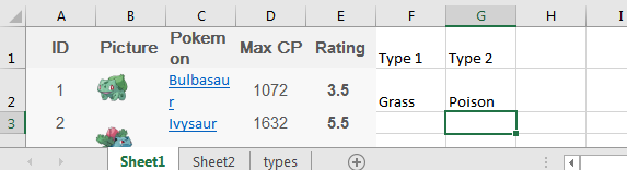
· You should now see the bulbasuar type 1 copied from your types sheet to your sheet 1.

· Repeat this for type 2, but the column index should be 3.

· You should now see both type 1 and 2 copied from the type table:

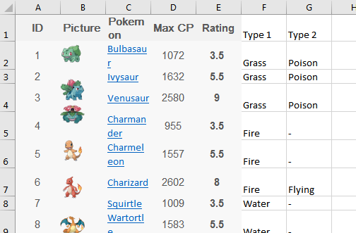
· Just copy that formula down to do the rest of the lookups.

· There is no need to do more for our exercise, but see that you now have more categories you could use if you created a new pivot table.

LAST STEP: Now just upload this to moodle.