Data Analysis and Mail Merge exercise
Overview:
Practice pivot tables and lookup commands and mail merge so that you can understand what power they have to save you work, and so that you know it can be easy to use. I am not expecting you to remember the mechanics, but rather to know how these features can help you.
· Why pivot tables: Pivot tables are very useful for quickly categorizing a list and getting totals. It is quick and powerful. You do need nice column headings and no merged cells, which can be tricky.
· Why Lookup: There will be times in your life that you are looking at 2 spreadsheets that you have to compare or match up in some way. Many people solve that manually, with lots of typing. Knowing the VLOOKUP commands power will help you match up columns from spreadsheets quickly.
· Why Mail Merge: Have you ever wanted to send the same letter or email to many people, but personalize it with their name? Maybe you needed to print labels to send a party invitation? Soon, you might want to send out resumes to every company in a list that you are targeting. You can send personalized individual emails or letters or labels to an entire list of people with a few keystrokes. For emails, it is helpful to have individual emails that are personalized and do not copy everyone on the list.
Requirements:
· Start with the spreadsheet provided in this link.
· Create One pivot table to count the number of companies of each location type in your list.
· Change the “person with company” sheet to use VLOOKUP to copy the company phone number for the company from “company with location”.
· Use of filter to choose only directors on the “person with company” sheet.
· Write a very cursory cover letter and do a mail merge of 4 letters
Movies:
|
Step |
Excel |
Open Office |
|
1 Overview and download |
||
|
2-3 Create the Pivot Table |
||
|
4 Lookup the phone number |
||
|
5 Filter |
||
|
6 Mail / Merge |
Detailed Instructions :
If you miss a step, just try the next one. Many of these steps do not depend upon the prior step completing properly.
STEP 1: Open the spreadsheet I created from the hoover database you
can access through Adelphi databases. Right
click on this link and choose to save link to your downloads
folder.
Step 2: Create a pivot table to count the number of
companies in each location
·
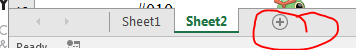
First add another sheet by clicking on the plus sign at
the bottom of your worksheet. You may need to maximize your window to see that
plus sign:
·
·
Navigate to the “company with location” tab by clicking
on the tab
·
Highlight the entire sheet by choosing the cell between A
and 1: ![]()
o
It was important that each column had a heading that was
not blank and did not have special characters.
Step 2 A – For Excel :
Actually creating the pivot table is different for Excel and Open
Office, so follow the Step 2 A for Open Office if you use that.
·
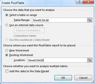
Insert a pivot table by choosing insert / pivot table.
·
If asked for a location, choose existing sheet and then
click on the new sheet and then a cell at the top of the new sheet. Not everyone will get this:
·
A pivot table field list will appear. You could arrange the fields in the pivot
table however you like.
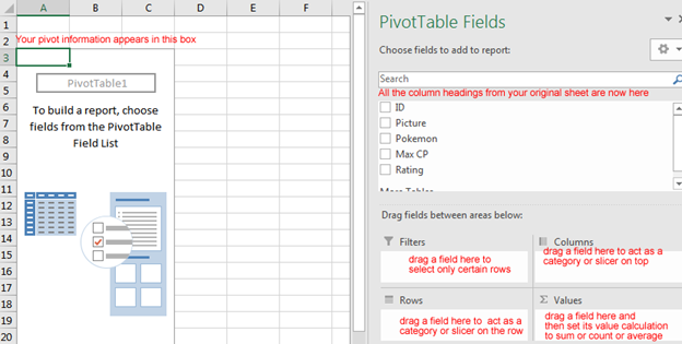
·
Now you can create a pivot table by dragging from the fields into the
filter, columns, rows and values boxes
·
To accomplish our goal, make this pivot table:
o
Drag location to the row box.
o
Drag company name to the values box.
o
Drag location type to the column box.
o
Drag Sales to the filter
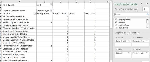
See how it summarizes your data with a few clicks. If you
had to sort and sum each category in the worksheet, it would take a very long
time. You can down arrow on the sales
(All) to choose just a few sales values to include in your table.
STEP 2A – For open office version 4 (If you use
Excel, skip down now to STEP 3)
·
Choose data menu, then data pilot option and then start,
and then enter to accept the current selection, and then see a pivot grid.
·
Drag the location button onto the row field section of
the pivot grid.
·
Drag the company name onto the data fields
·
Drag the location type into the column fields section.
·
Click on the more button and then click on the results to
spreadsheet icon and then click on sheet 2 and then a3 cell and then press
enter. (If you miss this, your pivot will be below your table.)
·
Then hit okay to accept the pivot grid which should look
like the screen below. Then you can
click on sheet 2 to see your pivot.
STEP 3: Play with the pivot table a little bit to
drill down
·
Drill down : Double click on a
number in your pivot table and see it open a new sheet with only those
companies that are represented in the cell you clicked.
STEP 4. Add phone number to the list of people in
each company using VLOOKUP
The person with company sheet has no address or phone
number. To get that, you will look up the “company with location” sheet to find
the row with the matching company name.
Click on “person with company” sheet
Under the location column, make a vlookup
formula
o
For Excel: From the formula ribbon, choose Insert
function, type vlookup, and double click it.
o
For Open Office: Insert menu / function option/ and then
down arrow until you find VLOOKUP and double click it and hit Next. Your 4
lookup parts will mean the same thing but have different labels from the
picture below.
·
Your lookup value should be the value that will match to
the lookup table, so in this example, click c2. The lookup table is the
“company with location” table, so click on the “company with location” sheet and then highlight columns a - g
. It always looks up from the left most value in the table you tell it to look
at.
·
After matching you want to return the phone number. It is
field number 7 (G is the 7th column if A is 1)
·
You only want exact matches , so choose FALSE on range lookup
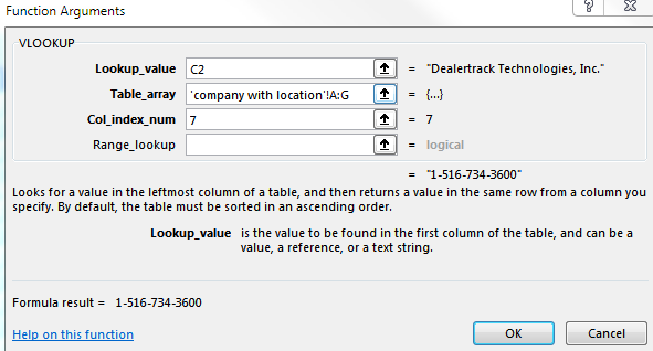
·
Just copy that formula down to do the rest of the
lookups.
STEP 5. Filter to show only people who are directors,
and copy that list to another sheet.
·
Highlight the first row
·
Choose filter (home ribbon, editing pane, sort and filter
option, choose filter )
·
Click the “all” filter box once and to unselect all
titles and then mark all titles starting with “director”
·
You should see fewer rows.
·
Select the entire sheet and right click to copy.
·
Add a new sheet and paste into that new sheet.
·
Name the sheet “final list”
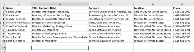
The final list should look like this:
STEP 6. Mail-Merge to create a personalized letter to
all the people on the “final list” sheet.
Overview: The letters should say just these 2
lines, with the values for first name, last name and company name merged in:
Step
6A for Office – Word and Excel:
The steps for
mail / merge are the same in every version of word, but the placement of the
options is different in every version. Please refer to the Learn Mail Merge
option in the “read / watch / do” section to see how to find the options
mentioned in the steps below. Some
versions have a mail/ merge wizard and others have the options on a ribbon.
1.
Open Word and create a
blank new document.
2.
Start mail / merge ->
select “letters”
3.
Select recipients -> select “use
existing list” and then find the ExcelAdvanced spreadsheet,
and then choose the final list sheet. If you never created the final list
sheet, you can use the “people” sheet. The ExcelAdvanced
sheet is likely to be in your downloads folder. In some systems, the downloads
folder is buried inside the “users” folder.
4.
Edit recipient list ->
Only choose 4 of the names. You can choose any 4 you like.
5.
Create your letter (just
type in the letter on the word document). Type the word “Dear” and then insert
the merged field “Name”. Then type “I want to work for “ and
insert the merged field “company”. Then type “. My resume is enclosed.”
I want to work for <<Company>>. My resume is enclosed.
6.
Preview results -> It
will show the names replacing the <<Name>> and you can scroll
through each letter.
7.
Save the document at this
point using File / Save.
8.
Finish and Merge -> Choose to “edit
individual records” and then choose all. Scroll through the document to see
that it holds 4
pages, one to each person you selected.
9.
Save the Letters that were
generated using File / Save.
Step
6B for Open Office Version 4
This is only
for open office, so skip if you have Word or Excel.
1.
Open writer and choose to
create a new document with file / new / text document
2.
Start writing the template
by using tools/ mail-merge wizard.
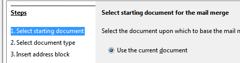
3.
Choose to use the current
document and click next.
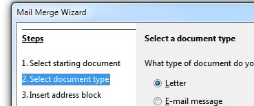
4.
Choose letter and click
next.
5.
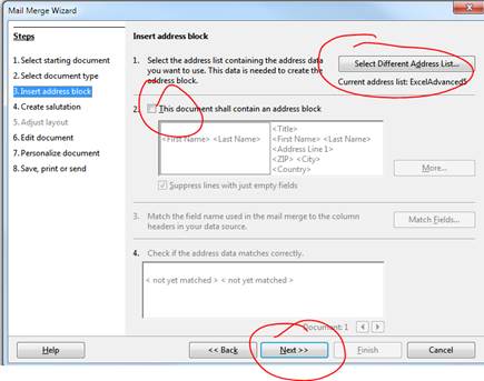
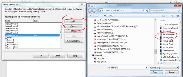
Choose “select different
address list” and then click Add. Navigate to the folder that has your ExcelAdvanced spreadsheet with a list of people to send
letters.
6.
Choose the final list
sheet. If you never created the final list sheet, you can use the “people”
sheet. The ExcelAdvanced sheet is likely to be in
your downloads folder. In some systems, the downloads folder is buried inside
the “users” folder. You do not have to
check “This document shall contain an address block.” Click Next.
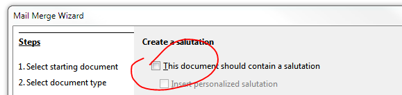
7.
You do not need a salutation
so choose to leave it blank, and click Next.
8.
Click Edit document.
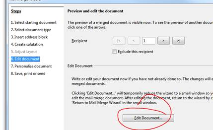
And see
9.
Create your letter (just
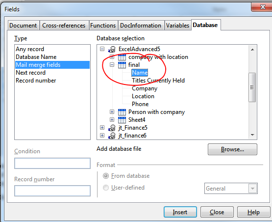
type in the letter on the word document). Type the word “Dear” and then insert
the merged field “Name”. Insert with
insert / fields / other and then choose the database tab and final ( or person with company) and then name. Then type “I want
to work for “ and insert the merged field “company”.
Then type “. My resume is enclosed.”
Dear <Name>:
I want to work for
<Company>. My resume is enclosed.
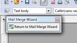
10.
Get back to the wizard by
clicking Return to Mail Merge
11.
Click Next on step 6 and
next on step 7.
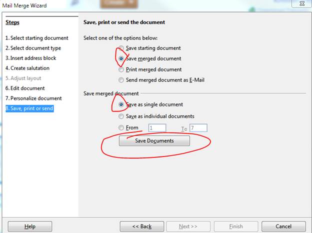
12.
Click to save the merged
document and save as a single document and then click the “save documents”
button.
13.
Name it Letters.
14.
File / Save the template
as Letter_Template.
LAST STEP: Now just upload the
excel spreadsheet, and the 2 word documents (the
template and the merged document) to moodle. If you had trouble, add another document
describing the problems you had. Be sure to tell me which step you reached. In
this exercise, you get stuck you can usually move on to the next step and skip
a step.